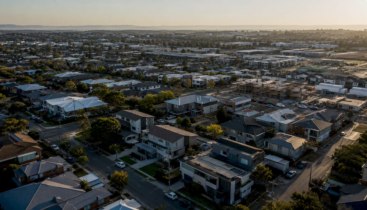
Why property cycles exist in Australian markets
Property markets cycle because demand and credit adjust quickly while housing supply responds slowly, producing repeated periods of shortage, then oversupply, then correction. The Reserve Bank of Australia’s empirical housing model confirms this: interest-rate movements, dwelling investment, rents and prices are tightly interlinked, and low rates alone explain a large share of recent price and construction surges. ABS data puts the total value of Australia’s residential dwelling stock at $12,772.6 billion across 11,495,200 dwellings as of the March quarter 2026 preliminary estimate, a figure that reflects decades of cyclical accumulation.
Three mechanics sit at the core of every property cycle:
- Inelastic short-run supply: you cannot build a suburb in six months. Construction lags mean prices rise sharply before new stock arrives.
- Credit and interest-rate swings: when borrowing becomes cheaper or easier, purchasing power jumps almost overnight, amplifying demand well beyond what supply can absorb.
- Population and demand shifts: migration surges, household formation changes, and shifting employment centres all alter demand faster than developers can respond.
Key takeaways
Property cycles exist because housing supply is structurally slow to respond while demand and credit can shift within months, producing repeated oscillations that no single policy lever or market participant can fully smooth out.
| Point | Details |
|---|---|
| Core mechanism | Inelastic supply plus credit swings create repeated boom-correction cycles in Australian property markets. |
| Four phases | Boom, downturn, stabilisation, and upturn each carry distinct signals: vacancy rates, approvals, credit growth, and price trends. |
| Cycle length varies | Investment cycles tend to run 7–10 years; development cycles often exceed 20 years, and local drivers mean cities can be in different phases simultaneously. |
| Timing is unreliable | RBA research warns that forecasting exact peaks and troughs is difficult; stress-testing cashflow and holding for a full cycle is more reliable than timing. |
| Wealthstacker | Free quarterly valuations, 15-year modelling, and suburb research tools help investors apply cycle awareness to real decisions. |
Table of Contents
- What is a property cycle, exactly?
- What are the four phases of the property cycle?
- What drives property cycles in Australia?
- Why inelastic supply and credit cycles produce oscillations
- How long do property cycles last, and why do they vary?
- What should buyers, sellers and investors actually do with this?
- How long-term modelling and suburb tracking make cycle awareness practical
- Wealthstacker: free tools for cycle-aware property investors
- Sources
What is a property cycle, exactly?
A property cycle is a repeating sequence of boom, downturn, stabilisation, and upturn across prices, rents, and construction activity. It is not a single event but a pattern that tends to recur, driven by the same structural mismatches each time.
Three distinct but overlapping cycles run simultaneously. The price cycle tracks median values and auction clearance rates. The construction or development cycle follows building approvals, completions, and land releases. The credit cycle measures mortgage growth, lending standards, and household debt. These three rarely peak at exactly the same moment, which is why reading any one of them in isolation can mislead.
The other critical distinction is scale. A national cycle reflects aggregate conditions: the RBA cash rate, broad credit availability, and national population growth. A local cycle reflects suburb-level vacancy rates, local employment, and the specific housing mix on offer. Sydney’s inner-ring apartment market and a regional Queensland mining town can be in opposite phases simultaneously. Understanding real estate cycles means holding both lenses at once.
Australia’s observed price peaks, as reported in ABS and RBA publications, show this clearly. The late 1980s boom and subsequent early-1990s correction, the mid-2000s surge, and the 2020–2022 pandemic-era run-up each had national characteristics but played out very differently across cities and suburbs.
What are the four phases of the property cycle?
CommBank’s consumer guide and RBA analysis both describe the same four-phase framework. Here is what each phase looks like on the ground.
Boom
Prices rise quickly, often accelerating quarter on quarter. Vacancy rates fall as rental demand outpaces supply. Building approvals climb as developers chase margins. Mortgage credit growth is strong and lending conditions are typically loose. Auction clearance rates sit well above long-run averages.

Indicators to watch: mortgage credit growth (published monthly by the RBA) and auction clearance rates (CoreLogic weekly data).
Downturn
Price growth stalls or reverses. Listings accumulate and days-on-market lengthen. Vacancies rise as new supply, approved during the boom, reaches completion. Lenders often tighten standards in response to rising arrears or regulatory pressure from APRA.
Indicators to watch: rental vacancy rates (published by SQM Research) and APRA’s monthly authorised deposit-taking institution statistics.
Stabilisation
Prices move sideways. Transaction volumes are low because buyers and sellers disagree on value. Developers pull back on new approvals. Rents may keep rising modestly if population growth continues, which gradually erodes the oversupply.
Indicators to watch: building approvals (ABS monthly series) and days-on-market trends.
Upturn
Vacancies tighten again as population growth absorbs the excess stock. Rents rise, improving yields and drawing investors back. Prices begin to lift, first in tightly held inner suburbs, then more broadly. Credit conditions often ease, either through rate cuts or loosened lending criteria.
Indicators to watch: rental yield trends and net overseas migration data (ABS).
| Indicator | Boom | Downturn | Stabilisation | Upturn |
|---|---|---|---|---|
| Price growth | Strong positive | Negative or flat | Flat | Early positive |
| Rental vacancy | Very low | Rising | Elevated | Falling |
| Building approvals | Rising sharply | Falling | Low | Beginning to rise |
| Mortgage credit growth | High | Slowing | Low | Recovering |
Pro Tip: *Combining a national indicator (cash rate direction, credit growth) with a suburb-level vacancy rate cuts false signals significantly.
What drives property cycles in Australia?
Supply inelasticity and construction lag
Housing supply cannot respond instantly to demand. Rezoning, development approvals, financing, and construction all take time, often years. When demand spikes, prices and rents rise sharply before a single new dwelling reaches the market. Academic analysis confirms that short-run supply inelasticity and financing variables together create oscillatory dynamics in both residential and commercial property cycles.
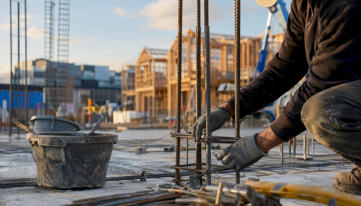
Signals to monitor: ABS dwelling approvals (monthly) and residential construction pipeline data.
Interest rates and credit conditions
The RBA’s empirical housing model finds that lower interest rates explain a large share of recent strength in both prices and construction. When the cash rate falls, borrowing capacity rises for every household simultaneously, pushing demand up across the board. The reverse is equally powerful: rapid rate rises in 2022–2023 cooled prices in most capital cities within months.
APRA’s role matters here too. Tightening serviceability buffers or restricting interest-only lending can dampen a boom even when the cash rate stays low. Historical RBA analysis shows that episodes of easing lending standards and rapid credit growth have amplified property booms and, in some cases, increased financial-system vulnerabilities.
Signals to monitor: RBA cash rate decisions and APRA’s monthly lending statistics.
Population growth and demographic change
Net overseas migration is one of the most direct demand drivers for housing. When migration surges, household formation accelerates faster than the construction pipeline can absorb. ABS dwelling stock data illustrates the scale: over 11.4 million dwellings serve a population whose growth rate fluctuates sharply with immigration policy and global conditions. The post-pandemic migration rebound contributed materially to the rental vacancy crisis of 2022–2024.
Signals to monitor: ABS net overseas migration estimates and household formation rates.
Government policy and tax settings
Negative gearing, capital gains tax discounts, first-home buyer grants, and stamp duty structures all affect the demand side. Supply-side policies, including zoning reform, infrastructure levies, and social housing investment, shape how quickly new stock can arrive. Policy changes can shift market sentiment almost immediately, even before a single dwelling is built or sold.
Signals to monitor: federal and state budget announcements affecting property tax settings.
Investor sentiment and behavioural factors
Fear of missing out (FOMO) during booms and fear of buying early (FOBE) during downturns amplify the underlying economic signals. Sentiment can push prices beyond what fundamentals justify and keep them depressed longer than supply-demand arithmetic would suggest. These behavioural factors do not create cycles on their own, but they widen the amplitude.
The interaction effect matters: low rates amplify demand and developer confidence simultaneously. Developers launch projects. By the time those projects complete, rates may have risen and demand softened, producing the oversupply that defines the next downturn. No single driver operates in isolation.
Why inelastic supply and credit cycles produce oscillations
The core mechanism is a timing mismatch. A demand shock, say a migration surge or a sharp rate cut, tightens vacancies and pushes rents up. Higher rents improve yields, attracting investors and developers. Developers respond by lodging approvals and commencing construction. But construction takes 18 months to three years. By the time those dwellings reach the market, the original demand shock may have faded, rates may have risen, or sentiment may have shifted. The result: a wave of new supply arrives into a softening market, vacancies rise, and prices correct.
This is the “cobweb” pattern described in the RBA’s housing model: supply responds with lags, and those lags produce repeated overshoots in both directions. It is not irrational behaviour by any individual actor. Developers respond rationally to price signals; the problem is that thousands of developers respond to the same signal at the same time, and the aggregate supply response arrives too late.
Academic research on Australian property cycles distinguishes between investment cycles (prices and transactions, roughly 7–10 years) and development cycles (land, approvals, construction capacity, often 20 or more years). The shorter investment cycle is more volatile and more visible to buyers and investors. The longer development cycle shapes the structural supply constraints that determine how severe each price correction becomes.
Historical Australian episodes illustrate the mechanism clearly. The late 1980s saw rapid credit expansion, strong migration, and rising prices. When the RBA tightened sharply and recession followed in the early 1990s, prices fell across most capital cities. The mid-2000s boom was similarly amplified by credit growth before the global financial crisis interrupted it. The 2020–2022 pandemic surge combined record-low rates, constrained supply chains, and a temporary collapse in new dwelling commencements, producing some of the fastest price growth on record.
| Variable | What it signals | Key Australian source |
|---|---|---|
| Dwelling approvals | Supply pipeline and developer confidence | ABS Building Approvals (monthly) |
| Rental vacancy rate | Tightness of current supply vs demand | SQM Research (monthly) |
| Mortgage credit growth | Demand amplification via credit | RBA Financial Aggregates (monthly) |
| Net overseas migration | Structural demand pressure | ABS Population Statistics (quarterly) |
| Cash rate | Cost of borrowing and investment hurdle rate | RBA cash rate history |
One important caveat: no single-factor model reliably predicts the next peak or trough. The RBA’s 2019 housing model is explicit about forecasting difficulty. Multi-factor explanations have stronger explanatory power than any single variable, but even they cannot pinpoint turning points with precision.
How long do property cycles last, and why do they vary?
Investment cycles in Australian residential property tend to run in the 7–10 year band, while development cycles are considerably longer, often exceeding 20 years, according to academic analysis of Australian property cycle determinants. These are tendencies, not fixed clocks. Actual length depends on the interaction of several forces.
Local population flows matter enormously. A suburb absorbing strong interstate migration will recover from oversupply faster than one losing residents to a regional shift. Local employment conditions, particularly in single-industry towns, can compress or extend cycles well beyond national averages. Housing mix also plays a role: high-density apartment markets tend to experience sharper supply responses and therefore more pronounced cycles than detached-housing markets where supply is more constrained.
National monetary policy moves uniformly but lands differently. This is why a 2019 RBA speech on housing and the economy emphasises that construction and price cycles are interlinked but not necessarily synchronous across cities.
A short checklist for diagnosing whether you are reading a local or national signal:
- Local signal: suburb vacancy rate moving independently of the city average; local building approvals diverging from state totals; local rental yield moving against the national trend.
- National signal: cash rate change; APRA-wide lending standard shift; national net overseas migration figure.
- Both at once: a national rate cut landing in a suburb with below-1% vacancy and a constrained land supply is the most powerful combination for price acceleration.
Thinking about a property investment timeline that aligns your holding period with expected cycle length is more useful than trying to pick the exact bottom.
What should buyers, sellers and investors actually do with this?
Cycle awareness is useful. Cycle timing is mostly a trap. The RBA and academic researchers are consistent on this: forecasting exact peaks and troughs is difficult even with sophisticated models, and investors who structure decisions around predicted turning points tend to underperform those who focus on fundamentals and holding periods.
The more productive approach is to use cycle knowledge for stress-testing rather than timing. Ask: if this property sits in a downturn for three years, can the cashflow sustain the mortgage? If rates rise 200 basis points from here, what happens to serviceability? These questions are answerable with data. “Will prices be higher in 18 months?” mostly is not.
Practical steps worth taking:
- Cashflow stress-testing: model the property at current rates plus 2–3 percentage points, and at vacancy rates 1–2 points above the current suburb average.
- Holding period alignment: match your expected hold to at least one full investment cycle (7–10 years minimum) so you are not forced to sell in a downturn.
- Suburb-level fundamentals: vacancy rate, rental yield, building approvals in the pipeline, and local employment base matter more than national headlines for individual property decisions.
- Geographic diversification: spreading across cities or regions reduces the risk of being concentrated in a single phase. Portfolio diversification strategies that span different markets reduce cycle-specific concentration risk.
- Monitor actively: set a quarterly review cadence covering vacancy, approvals, credit growth, and the cash rate.
Pro Tip: Run scenario models rather than point forecasts. If the portfolio survives all three, you are positioned for cycle resilience rather than cycle timing. Investment property forecasting methods that use multi-scenario modelling are far more reliable than single-path projections.
How long-term modelling and suburb tracking make cycle awareness practical
Understanding why property cycles exist is one thing. Applying that understanding to a specific suburb, a specific budget, and a specific life stage is where most investors get stuck. The gap between knowing the mechanism and making a decision is usually a data and modelling problem.
Fifteen-year modelling is particularly useful here. Over a horizon that spans at least one full investment cycle and potentially two, short-term noise matters less and structural drivers, population growth, supply constraints, income growth, dominate the outcome. Scenario stress-testing across different interest-rate paths and vacancy assumptions gives a realistic picture of portfolio resilience rather than a single optimistic projection.
Typical use cases where this kind of modelling adds real value:
- Comparing rentvesting versus buying under different rate environments, where the answer changes materially depending on assumptions about rental growth and capital appreciation.
- Testing negative-equity risk: at what price fall does the loan-to-value ratio breach a threshold that triggers margin calls or forces a sale?
- Suburb-level vacancy and rent scenarios: which suburbs have the supply pipeline and population dynamics to sustain rent growth through a national downturn?
The honest caveat is that modelling reduces uncertainty; it does not eliminate it. No tool predicts exact cycle peaks or troughs. What good modelling does is replace gut-feel timing with structured scenario thinking, which is a meaningful improvement for most investors.
Wealthstacker: free tools for cycle-aware property investors
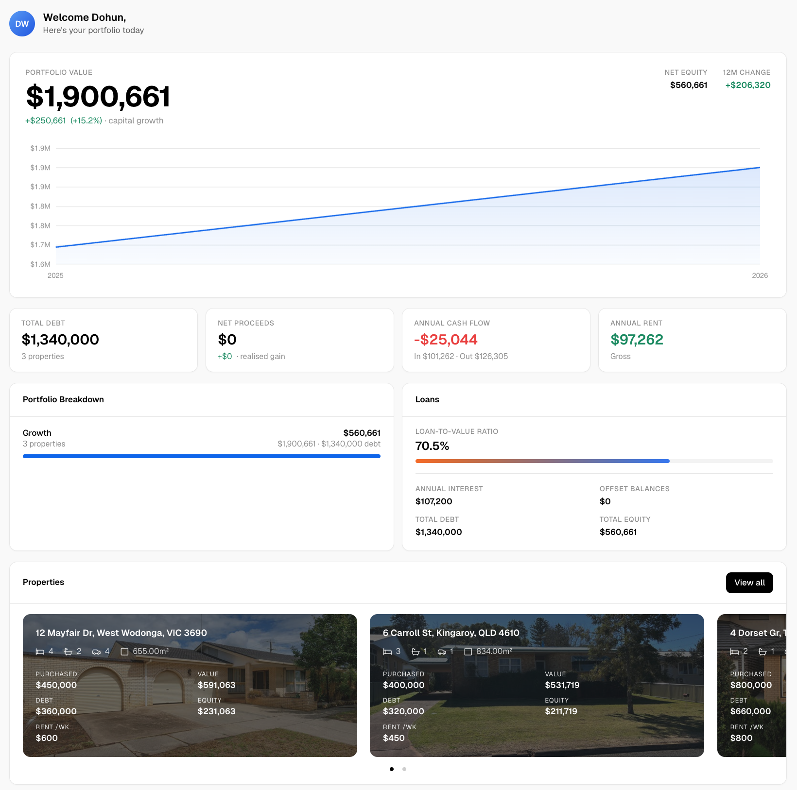
Wealthstacker gives you a free property investment toolkit built for exactly the kind of cycle-aware, long-term thinking this article describes. The platform provides automated quarterly property valuations at no cost, a portfolio tracking dashboard, and 15-year investment modelling tools that let you compare rentvesting and buying scenarios across different interest-rate and vacancy assumptions. An AI-powered investment chat assistant and suburb-level market research tools mean you can move from national cycle awareness to suburb-specific analysis without switching platforms.
The goal is not to help you time the market. It is to give you the data and modelling to make decisions that hold up across a full cycle, not just in the conditions that exist today. Visit Wealthstacker to access the free toolkit and see how 15-year scenario modelling applies to your own situation. This content is general information only and does not constitute personal financial advice. For advice tailored to your circumstances, consult a licensed financial adviser.
Sources
The following sources underpin the claims in this article and are worth bookmarking for ongoing research.
- RDP 2019-01: A model of the Australian housing market (RBA)
- Examining the macroeconomic determinants of property cycles in Australia
- Total value of dwellings, Australia (ABS) — latest release
- What is a property cycle? (CommBank)
This article is general information, not a substitute for advice from a qualified financial advisor. Consult a qualified financial professional about your own circumstances before acting on anything here.
Recommended
- Passive property investment strategies for Australian professionals | WealthStacker
- Portfolio performance metrics checklist: Australian investor guide | WealthStacker
- Property investment checklist for beginners: 2026 guide | WealthStacker
- Why dual income households invest in property faster | WealthStacker