
Depreciation Schedule Cost To Enter In WealthStacker For Australia
Inside a WealthStacker forecast, “depreciation schedule cost” refers to the projected Division 43 and Division 40 deduction figures you set as model inputs, not a fee you pay a quantity surveyor. Get this input right and three things follow: confirm your Division 43 rate, decide whether Division 40 runs on diminishing value or prime cost, and check your quarterly period maths isn’t silently wrong.
TL;DR:
- Properly modeling depreciation requires distinct streams for Division 43 and Division 40, with correct methods significantly affecting early cash flow and tax benefits.
- Using a depreciations schedule from a qualified quantity surveyor typically costs a few hundred dollars, with first-year deductions often covering the schedule fee within months.
- Accurate quarterly depreciation calculations must avoid dividing annual rates directly, instead applying the correct compounding formula to reflect true deductions.
- Higher early depreciation claims improve after-tax cash flow and lender serviceability but can increase capital gains tax upon sale due to a reduced cost base.
- For properties built after 1987 or with recent capital works, commissioning a depreciation schedule provides long-term benefits that outweigh the initial cost, especially when validated through forecast models.
Table of Contents
- What the depreciation input includes: Division 43 and Division 40 explained
- Typical depreciation schedule cost and how the fee behaves in a model
- How to model depreciation correctly in a quarterly forecast
- How different depreciation assumptions change cashflow and borrowing power
- Who actually needs a depreciation schedule, and why
- What drives the cost of a depreciation schedule up or down
- What a depreciation schedule typically itemises
- Choosing a professional to prepare your schedule
- Weighing the fee against the tax savings
- Running these numbers inside WealthStacker
- Sources
What the depreciation input includes: Division 43 and Division 40 explained
Every projection you run needs two separate depreciation streams, and conflating them is the most common modelling mistake we see.
Division 43 (capital works) covers the building’s structure: brick, concrete, fixed tiling, built-in wardrobes. The standard modelling convention is prime cost at 2.5%-and-diminishing-value-methods/) of the original construction cost, straight line, for up to 40 years from the completion date. That’s an ATO convention, not a guess, and it’s the figure most forecasting tools default to because it rarely changes once the build cost is known.
Division 40 (plant and equipment) covers items with a shorter effective life: hot water systems, carpets, air-conditioning units, blinds. Here you’ve got a genuine choice between two methods:
- Prime cost spreads the deduction evenly across the item’s effective life.
- Diminishing value front-loads deductions, giving you a bigger claim in years one and two, then tapering off.
The method you pick doesn’t change the total amount depreciated over an asset’s life. It changes when you get it, and that timing shift is what actually moves your early cashflow, your serviceability numbers, and how a lender reads your application in year one versus year five.
Typical depreciation schedule cost and how the fee behaves in a model
A tax depreciation schedule from a quantity surveyor typically costs a few hundred dollars for a standard residential property, according to figures reported by Property Investment Professionals. That fee is generally tax deductible in the year you pay it, and because first-year deductions on a newer property can run into several thousand dollars, the fee routinely pays for itself well within the first tax return.
Rough first-year deduction bands look like this:
-
New or near-new properties: often the highest combined Division 43 and Division 40 claims, since construction cost is fresh and plant items haven’t depreciated yet.
-
Established properties (10 to 20 years old): Division 43 may still apply if built after September 1987, but Division 40 claims shrink as existing plant ages out.
-
Older properties with no capital works eligibility: Division 40 on any newly installed plant is usually all that’s left to claim.
At common marginal tax rates, a first-year deduction in the thousands can translate into a meaningful reduction in tax payable, which is exactly the kind of swing that belongs inside a proper investment modelling exercise rather than a rough mental estimate.
Here’s the practical split: use an internal projected schedule, built from published effective lives and construction cost estimates, when you’re forecasting scenarios in a tool like WealthStacker. Commission an actual QS report only when you need a defensible figure for your tax return.
How to model depreciation correctly in a quarterly forecast
Most depreciation errors in forecasting models aren’t conceptual, they’re arithmetic. Follow these steps and you’ll avoid the ones that actually distort a forecast.
- Decompound diminishing value rates properly. Never divide an annual DV rate by four to get a quarterly figure. The correct approach uses
period_rate = 1 − (1 − annual_rate)^(1/periods_per_year), a formula confirmed in ATO guidance on depreciation methods. Simple division systematically understates early charges. - Set a binary flag for possession. Depreciation shouldn’t start ticking over the moment a property appears in your model. Flag the actual completion or settlement date, and hold the depreciation calculation off until that point. Off-the-plan purchases are where this trips people up most, since the purchase date and the completion date can sit a year or more apart.
- Handle new additions and ongoing capex separately. A new hot water system installed in year four starts its own depreciation clock; it doesn’t get blended into the original Division 40 pool. Keep additions as discrete line items so your total depreciation base always matches what’s actually been installed.
- Write off residual value at end of effective life. Diminishing value balances asymptotically approach zero but never quite hit it. Build an explicit write-off rule so residuals don’t compound pointlessly across a 15-year forecast.
Common errors worth checking for: applying Division 43 to a pre-1987 building with no eligible capital works, using the wrong effective life table for plant items, and forgetting that accumulated Division 43 claims reduce your cost base for capital gains purposes on sale.
Pro Tip: Once a quarter, pull your model’s cumulative depreciation total and sanity-check it against a straight back-of-envelope calculation, construction cost multiplied by 2.5%, times years elapsed. If the numbers diverge by more than a rounding error, something in your period maths has broken.
How different depreciation assumptions change cashflow and borrowing power
Run three scenarios before you commit to a purchase decision, not one.
- Base case: realistic Division 40/43 split based on comparable properties, prime cost method.
- Conservative case: lower Division 40 allocation, prime cost throughout, longer holding period.
- Aggressive case: higher Division 40 share, diminishing value method, shorter anticipated hold.
Higher early depreciation increases your tax refund, which improves after-tax cashflow, and some lenders will factor stronger net rental yield into their serviceability assessment. But there’s a trade-off on the back end: every dollar of Division 43 you claim reduces your cost base, which increases the capital gain, and therefore the CGT bill, when you eventually sell. A model that shows glowing early cashflow but ignores this is quietly overstating your long-term return.
Compare these outputs across all three scenarios:
| Output | What to watch for |
|---|---|
| After-tax monthly cashflow | Gap between conservative and aggressive can be hundreds of dollars a month in year one |
| Lender serviceability ratio | Higher depreciation improves this, but banks apply their own haircuts |
| IRR / NPV over the hold | Method choice rarely moves this materially; holding period does |
| Projected net worth at 10 to 15 years | Should account for reduced CGT cost base, not just cumulative deductions claimed |
When you take these numbers to a lender for a borrowing power conversation, use the conservative scenario, not the aggressive one. Banks tend to discount projected tax benefits anyway, and turning up with an inflated serviceability figure built on best-case diminishing value assumptions is a fast way to lose credibility with a broker. For a fuller breakdown of which metrics matter across a long hold, our guide to investment property forecasting methods walks through the sensitivity checklist in more detail.
Who actually needs a depreciation schedule, and why
Not every property owner needs to think about this. If you own your own home and never rent it out, depreciation on the building and fixtures isn’t claimable, so the question is moot. It becomes relevant the moment a property starts producing rental income, whether that’s a dedicated investment purchase or a rentvestor’s arrangement where you rent out a property you own while renting somewhere else yourself.
Property investors need a depreciation projection for two distinct reasons that often get blurred together. The first is compliance: at tax time, you need defensible figures to include in your return, which is where a QS-prepared schedule earns its keep. The second is decision-making: before you buy, before you decide whether to renovate, before you choose how long to hold, you need a forecast of what depreciation will do to your cashflow over the coming years. That second use case is squarely a modelling exercise, and it’s the one this article, and WealthStacker’s tools, are built around.
Joint owners, self-managed super fund property purchases, and small property syndicates all have their own wrinkles around who claims what share of a depreciation deduction, but the underlying mechanics of Division 43 and Division 40 don’t change. What changes is how the deduction gets split and reported.
What drives the cost of a depreciation schedule up or down
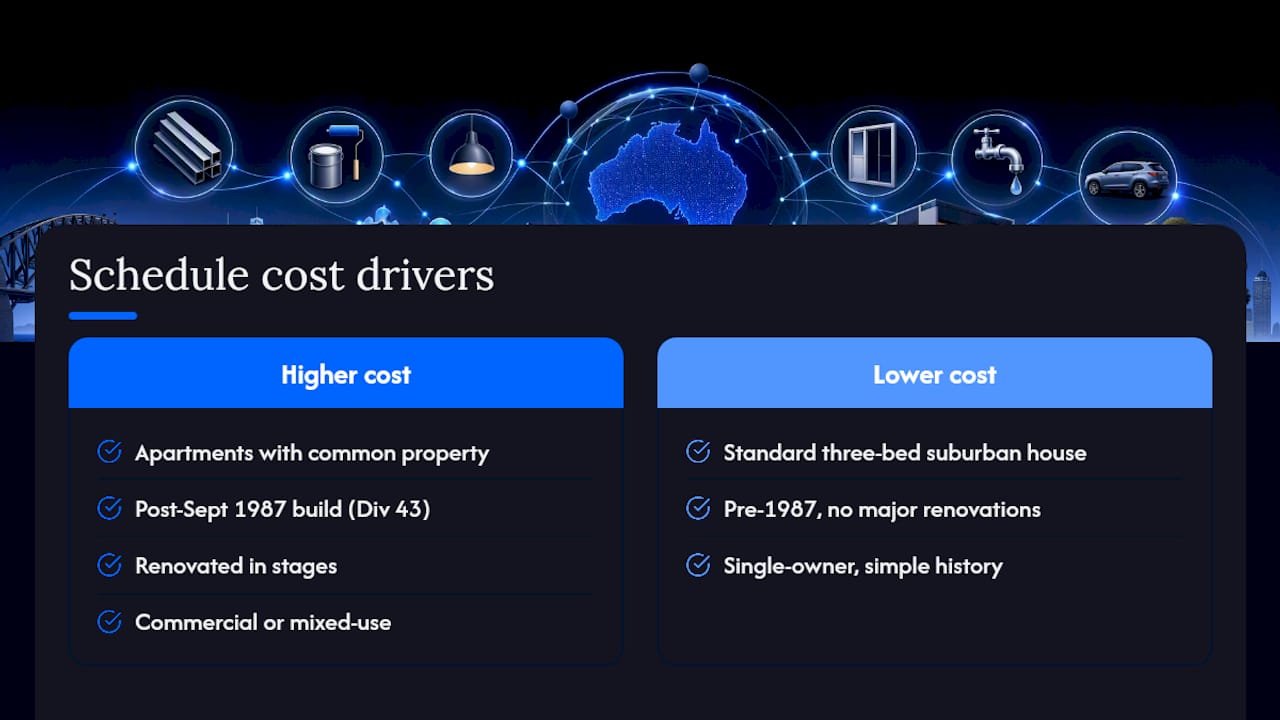
Property type is the biggest lever. A standard three-bedroom house on a suburban block is the cheapest and fastest schedule to produce, because there’s a limited, well-understood set of plant and equipment items to catalogue. Apartments in larger complexes cost more, because a quantity surveyor also has to account for a share of common property, lifts, shared air-conditioning plant, security systems, which requires liaising with the body corporate or strata manager.
Age matters almost as much. A property built after September 1987 carries Division 43 eligibility, so there’s more to calculate and more value in getting the schedule done. A property built well before that date, with no substantial renovations since, may have little to nothing worth claiming under Division 43, which can actually make the schedule cheaper because there’s less to assess, but also less useful.
Complexity is the third factor, and it’s the one people underestimate. A property that’s been renovated in stages over several owners needs the QS to reconstruct a history of what was replaced and when, since each renovation resets the depreciation clock on those specific items. Commercial or mixed-use properties add another layer again, with different effective life tables applying to fit-out items depending on the tenant’s industry.
Location can nudge the fee slightly too. Firms operating in regional areas sometimes charge a site-visit premium if a physical inspection is required and the property sits some distance from their base.
What a depreciation schedule typically itemises
A standard schedule breaks the property into its Division 43 capital works component and its Division 40 plant and equipment component, then itemises the latter in detail. Expect line items covering hot water systems, ovens, cooktops, dishwashers, carpets and floating floors, blinds and curtains, ceiling fans, garage door motors, and smoke alarms, each assigned an effective life drawn from the ATO’s determination tables.
For newer properties, the schedule usually includes a construction cost breakdown supporting the Division 43 claim, sometimes estimated by the quantity surveyor where original builder invoices aren’t available. For renovated properties, it should separately itemise what was replaced during the renovation, since those items start a fresh depreciation clock from the renovation date rather than the original build date.
A well-prepared schedule also projects forward, typically showing year-by-year deductions for the life of each asset, often presented under both the prime cost and diminishing value methods so the owner or their accountant can choose. This forward projection is precisely the kind of output you’d want to feed into a longer-term cashflow model, translating a static compliance document into an assumption you can actually stress-test.
Choosing a professional to prepare your schedule
The work of estimating construction costs and assigning effective lives for tax purposes sits with quantity surveyors, and the ATO specifically recognises this profession as qualified to estimate historical construction costs where original invoices aren’t available. An accountant generally isn’t the right person to prepare the schedule itself, though they’ll use its output when they lodge your return.
Look for membership of the Australian Institute of Quantity Surveyors, a track record specifically in residential investment property (commercial and residential depreciation work draw on different effective life tables), and a firm willing to explain their construction cost estimate methodology rather than just handing over a number. A reasonable firm will also offer a fee guarantee of some kind, commonly a promise that if the deductions identified don’t exceed the fee charged, you don’t pay.
Red flags are fairly consistent across the industry: firms quoting a price without first asking basic questions about the property’s age and history, schedules that arrive within a day or two of a phone call with no site inspection for a property that clearly warrants one, and anyone reluctant to put their AIQS membership number on the engagement letter. For useful background on where the line sits between a compliance schedule and a forecasting input, this guide on tax write-offs for investment property covers the practical distinction well.
Weighing the fee against the tax savings
Set against a $385 to $770 fee, the maths on a new or near-new investment property is rarely close. First-year Division 40 and Division 43 deductions on a recently built property commonly run into the thousands of dollars, and at typical marginal tax rates, that translates into a tax saving that dwarfs the schedule’s cost in year one alone, then keeps paying out annually for years afterward.
The calculation gets less clear-cut on older established properties with no capital works eligibility and minimal remaining plant value. Here, the total deductions available over the schedule’s useful life might only be a few hundred dollars a year, and an investor needs to genuinely weigh whether the fee is worth committing to versus simply using conservative default assumptions inside a forecasting model until a renovation or improvement changes the picture.
The general rule holds for most investors: if the property was built after 1987, or has had any meaningful capital works or plant replacement since, get the schedule. The fee is deductible, the payback period is typically under twelve months, and the ongoing deductions compound in value over a long hold. Where doubt exists, a quick internal estimate using standard effective life tables, run through a forecast, will usually tell you whether commissioning the full schedule is worthwhile.
Running these numbers inside WealthStacker
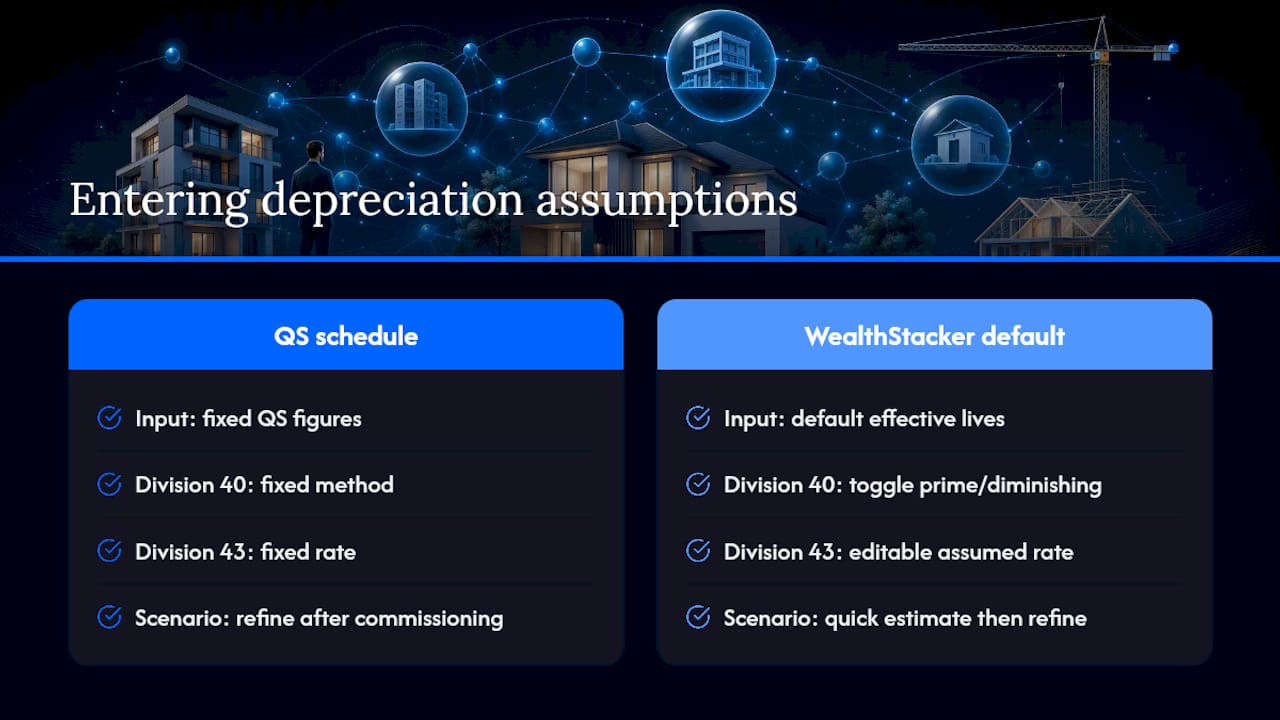
Once you know your Division 40 and Division 43 assumptions, the next problem is getting them into a cashflow model without rebuilding a spreadsheet from scratch every time something changes. Wealthstacker’s toolkit is built around exactly this gap: automated quarterly valuations feed directly into your net worth projections, and the modelling engine includes toggles for Division 40 method (prime cost or diminishing value) and Division 43 rate, so you’re not stuck guessing at quarterly decompounding formulas by hand.
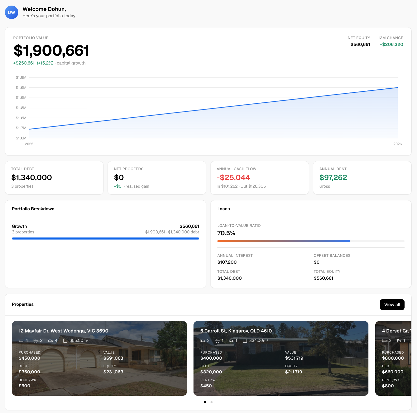
If you’ve already got a QS-prepared schedule, you can enter its Division 40 and Division 43 figures as fixed inputs. If you’re still deciding whether a property’s worth pursuing, use WealthStacker’s default effective life assumptions to run a quick estimate first, then refine it once you commission the real thing. Either way, the sensitivity dashboard lets you flick between the base, conservative, and aggressive scenarios described earlier and watch the effect ripple through your after-tax cashflow, your borrowing power estimate, and your 15-year net worth projection in real time.
For rentvestors comparing a purchase against continuing to rent, the same depreciation assumptions plug straight into the buy-versus-rent comparison tool, so you’re weighing a realistic after-tax picture rather than a pre-tax approximation that flatters ownership. Head to WealthStacker to set up a free forecast, load your property details, and see exactly how your depreciation assumptions move the numbers that actually matter for your next decision.
This article is general information, not a substitute for advice from a qualified financial advisor. Consult a qualified financial professional about your own circumstances before acting on anything here.